Optimization for babies - Part 2: Simulated annealing in R
In the last post I outlined the basics of optimization and one of the simplest optimization techniques - gradient descent. However, gradient descent has a major flaw - it fails when faced with multiple minimas (or maximas).
Let's take an example to understand. Suppose our objective function is

#Objective Function
obj_fun<-function(x)
{
return(x*sin(x))
}
#Graphical representation of objective function
valuesx<-c(1:50)
obj_out<-obj_fun(valuesx)
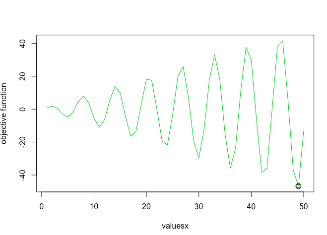
plot(x=valuesx,y=obj_out,typ='l', col=3)
sprintf("minimum value of objective function: %f",min(obj_out))
sprintf("minimum x: %i",valuesx[obj_out==min(obj_out)])
points(x=valuesx[obj_out==min(obj_out)],y=min(obj_out), col=1, cex=2)
This function has multiple low points (or rather multiple points where slope is equal to zero), but its true minimum is a x = 49.
(Note: In this example we have restricted the sample space between 1-50. For this sample space the minima is at 49. However, in an unbounded sample space the minima could be different)
Because of multiple low points, gradient descent stops when it encounters a point with slope = 0. But this might not be the true minimum. For example - when we use gradient descent to solve the function, the algorithm gets "stuck" in a local minima
out<-grad_descent(x=20, alpha=0.1,max_iter =100)
points(x=out$x,y=out$f_x) # Plot optimisation plots
(Note here I used a self-written custom gradient descent function. To understand the details of the code check out my previous post about gradient descent)
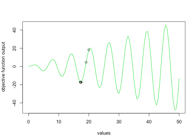
As you can see gradient descent stopped at local minima of 17 but failed to find global minima. One way to solve this problem is using simulated annealing optimization
What is Simulated Annealing optimization?
Simulated annealing is an optimization technique based on the chemistry process of annealing. This optimization method is mainly popular because it does not reject bad solutions but rather accepts them with a lower probability. This allows for the algorithm to not get stuck in local optimum and find global optimums.
In Simulated Annealing, we basically run the solver until it gets stuck. We then heat the system (increase parameter T), making it jump over local humps (accept bad solutions). Temperature is slowly reduced. With each iteration of reduced temperature, bad solutions are accepted with lesser probability. That means lower the temperature lower is the chance of accepting bad solutions. The temperature is a way of controlling the fraction of steps that are taken that don’t improve the objective function. The temperature is gradually reduced according to a cooling schedule. The lower the temperature, the more it acts like a greedy algorithm. We reduce temperature and run the solver again until it stops. We repeat this over and over until we find the global minimum.
Okay that's a lot of theoretical stuff, but how do I put into practice?
Let's break it down into pseudo code. The annealing optimization can basically be broken down into three steps
STEP 1 - Start with an initial solution s0. Calculate the objective function value for s0 (f0). Because at this stage we don't have any solutions yet current and best state are same as initial state
STEP 2 - Next, find a random neighbor (sn) of current state (sc) and calculate fn.
STEP 3 - If fn is less than best state (fb) accept it and assign it to fc. If fn is not less than fb, accept it only if temperature allows. We use the metropolis acceptance criterion to decide probability of accepting a bad solution. Remember as the temperature decreases the probability of accepting a bad solution also decreases.
Repeat STEP 1-3 until temperature is extremely low or max iterations are reached
#Define objective function
obj_fun<-function(x)
{
  return(x*sin(x))
}

#Find neighbor function
find_neighbor<-function(s){
  s<-sample.int(50,1)
  return(s)
}


#Define simulated annealing function
#obj_func = function to be optimized
#s0 = initial state
#step = step size
#find neighbor = function to find the next solution to test from the sample space

simulate_annealing_function<-function(obj_fun,s0=0,step=0.01,find_neighbor)
{

  #Initialize
  #s stands for state
  #f stands for function value
  #b stands for best
  #c stands for current
  #n stands for neighbor

  s_b<-s0
  s_c<-s0
  s_n<-s0

  f_c<-obj_fun(s_c)
  f_b<-f_c
  f_n<-f_c
  k=1
  Temp<-(1-step)^k

  while (Temp>0.000001)
  {
    #Set Temperature. As iteration increases temperature decreases (slowly)
    Temp<-(1-step)^k

    #consider a random neighbor
    s_n<-find_neighbor(s_c)        #Here I have written a custom find neighbor function

    f_n<-obj_fun(s_n)                 #Find objective function value for neighbor state
    #print(f_n)

    #update current state
    #Accept neighbor or jump to neighbor point only if neighbor is "good"
    #i.e value of neighbor function is less than current neighbor
    #OR if neighbor is bad then accept it only based on schedule
    #probability. Higher the temp more chance of poor solution being accepted
    if(( f_n>f_c) | runif(1,0,1)<exp(-(f_n-f_c)/Temp))
    {
      s_c<-s_n
      f_c<-f_n
    }

    #update best state
    if(f_n<f_b)
    {
      s_b<-s_n
      f_b<-f_n
    }
    k=k+1
  }

  #return best state and best objective function value
  print("best state")
  print(f_b)
  return(s_b)
}
Let's test the function and see the results
#Call function
s0=20   #Initial starting point
sa_out<-simulate_annealing_function(obj_fun = obj_fun,s0 = s0, find_neighbor = find_neighbor)

#Plot function
points(x=sa_out[1],y=sa_out[2],cex=1.5)
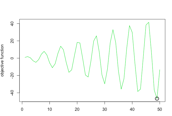
As you can see simulated annealing successfully finds the global minima!
More Reading: