Optimization for babies - Part 1: Gradient Descent in R
Mathematical optimization or mathematical programming is the selection of a best element, with regard to some criterion, from some set of available alternatives. Strangely enough optimization is one of the most common but also one of the hardest real-life problems to solve! Personally I love optimization because it's like trying to unlock a giant puzzle. But finding the right optimization function to solve your problem is half the battle! Optimizing the optimization function is real!!
Before we talk about some popular techniques let's first understand the basics
What is optimization?
Optimization is the process of trying multiple selections from a sample space to select the best one. A mathematical optimization problem consists of three main parts
- Objective - the function, equation or metric we are trying to optimize (i.e minimize or maximize). Real world examples include maximize revenue, minimize cost, find shortest path between two cities and so on
- Decision space - the sample space of solutions that we sift through to find the best solution
- Constraints - rules or limitations that apply to the decision variables
Optimization Techniques - Gradient Descent
Gradient descent is the most popular optimization method. Intuitively, you can understand the logic behind gradient descent as an algorithm that tries to move towards the minimum by moving (in the sample space) in the direction of the steepest slope downhill. Imagine one day you wake up and you are shrunk to the size of an ant. You find yourself stuck on the edges of a giant uneven bowl and you are trying to get to the food at the bottom.
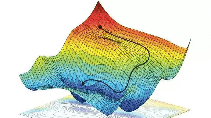
Now you don't know which direction is the bottom because obviously your brain has shrunk too so you are stupid. But you remember this blog and realize you'll get to the bottom as long as you only keep going downhill. But there are so many directions that seem to go downhill. Which one will get you down fastest? The answer is the steepest slope! If you keep sliding downhill along the steepest slope at one point you are going to reach flat ground and have no slope to slide down. That has to be the bottom or the minimum!
Okay now that we understand the logic behind it let's try the math
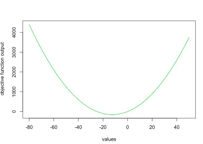
The basic idea is to define the objective function , take the first order derivative also known as the cost function and then use this function to take the next step in the sample space. Let's take a very simple function

#Define objective function
obj_fun<-function(x)
{
  return(x^2+25*x)
}

#Graphical representation
valuesx<-c(-80:50)
obj_out<-obj_fun(valuesx)
plot(x=valuesx,y=obj_out,typ='l', col=3, xlab = 'values', ylab=' objective function output')
Doing some simple calculus the cost function is

Using the logic of gradient descent we use this cost function to jump to the next best solution set (x) using the following

where alpha is the learning rate or the step size to take in each iteration
#Define cost function
cost<-function(x){
  return(2*x+25)
}

#Gradient descent function
grad_desc<-function(x = 0.1, alpha = 0.6, conv=0.001, max_iter=100)
{
  #alpha = learning rate or step size
  #conv = maximum improvement from previous iteration
  #max_iter = stopping iterations

  xtrace <- x
  ftrace <- obj_fun(x)
  diff=obj_fun(x)
  iter=1

  #Search for solution until max iterations are reached or improvement is very minimal
  while (iter<max_iter & diff>conv) {
    prev_out<-obj_fun(x)
    x <- x - alpha * cost(x)
    new_out<-obj_fun(x)
    diff=prev_out-new_out

    xtrace <- c(xtrace,x)
    ftrace <- c(ftrace,obj_fun(x))
    iter=iter+1
  }

  data.frame(
    "x" = xtrace,
    "f_x" = ftrace
  )
}
Let's run and test the function
#Test optimisation function
out<-grad(x=20, alpha=0.1 ,max_iter =100)

#Minimum
print(tail(out,n=1)
#-12.45977 -156.2484
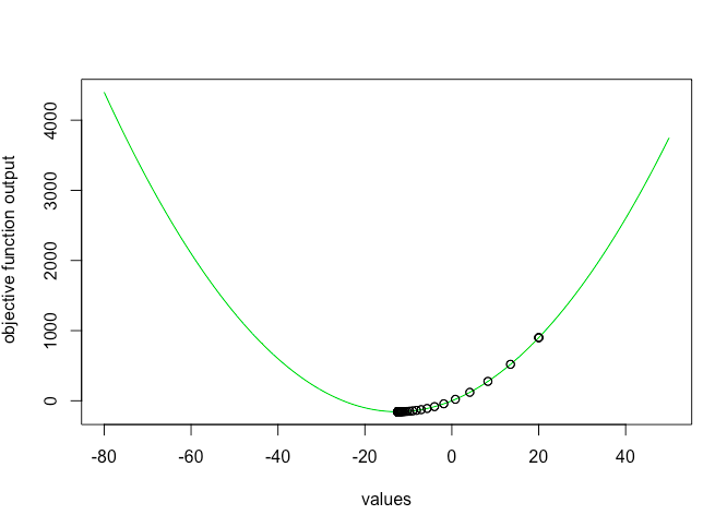
Wohoo! You succesfully implemented a gradient descent algorithm and found the minima of a function. Tracing the output shows how function reached the minima
#Plot of output
plot(x=valuesx,y=obj_out,typ='l', col=3, xlab = 'values', ylab=' objective function output')
points(x=out$x,y=out$f_x)
Gradient descent is great algorithm when we have only one minima or maxima, however it gets stuck in local minimas when we have more than one valleys or peaks. Check out part 2 to see how we can tackle this problem!
More Reading: